SOLAR ACTIVITY SYNCHRONISATION / MODULATION

THIS WEB PAGE WILL BE UPDATED WITH LATEST AVAILABLE INFORMATION

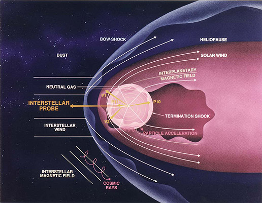
                                Fig. 1 & 1a

Nasa video shows the flux loop engulfs major magnetospheres, and goes all the way to heliopause: Magnetic cloud
 

Recent observations indicate that magnetic field lines of magnetic clouds do remain connected to the Sun [Larson et al., 1997]. nrl.navy.mil/prediction/storms
...that the electrical current and the magnetic field are parallel and proportional in strength everywhere within its volume.  Lepping et al
and http://wind.nasa.gov/mfi/mag_cloud_pub1.html
Magnetic cloud (Fig. 2) shows heavier particles move forward (orange shading) but ... the electrical current and the magnetic field are parallel and proportional in strength everywhere within its volume ......the electrical current and the magnetic field of magnetic clouds do remain connected to the Sun as quoted above.

Fig 2

R.P. LEPPING et al, from Laboratory for Solar and Space Physics NASA-Goddard Space Flight Center

A summary of WIND magnetic clouds for years 1995-2003 : model-fitted parameters, associated errors and classifications

MCs (magnetic clouds) are 1/4AU in diameter, have a broad distribution of axial directions with a slight preference for alignment with the Y-axis(GSE), have axial fluxes of 10^21Mx, have axial current densities of about 2μA/km2, and carry a total axial current  of about a billion amps.

Hironori Shimazua,b,c, MotohikoTanaka: A flux rope requires a large electric current to maintain its magnetic field.....the flux rope is maintained only by the electron current. This assumption is reasonable because the proton current alone cannot make a structure smaller than the proton cyclotron radius. Protons are assumed to have no bulk drift except for thermal motion.....In the initial equilibrium, the electrons move along the magnetic field lines, and this electric current generates the magnetic field of the flux rope.

A.A. van Ballegooijen, E.E. DeLuca: The high conductivity of plasma implies that the electric currents can be maintained for a long period of time.

Implication of the above is that electric current / magnetic field are still connected to the Sun, even if mass ejection has stopped some time before, and ejected mass of heavier particles may have moved some distance (Fig. 2 orange shaded area). During an impact with a magnetosphere the above electric current / magnetic field will be affected, and since they are still attached to the Sun, feedback will arise.

Electric current for its propagation will utilise any electrons (solar wind etc) that happen to be in path of highest conductivity/lowest resistance (solar wind  is of near infinite conductivity, very low resistance). While mass ejection lasts (for few hours) the current will start and close at the CME's origin, but as mass ejection ends the current loop becomes independent from its initial location, as long there are enough electrons in corona (to propagate electric field around the loop) the electric current will flow within force-free structure. The whole process, from a single CME, may lasts for some months, until CME hits heliopause:NASA video. The CME's play critical role in the solar magnetic flux polarity reversals.

Result of a possible electro-magnetic feedback within heliosphere is shown in correlation between solar activity and the two major magnetospheres' ( Jupiter & Saturn ) orbital properties. Configuration of the magnetic field within the heliosphere is complex and depends on number of factors. As a planet with magnetosphere moves along their orbits, magneto-tail is always in direction away from the sun. Both magnetic field and electric current within CME are partially short-circuited by the Jupiter / Saturn magnetospheres through process  of reconnection. The effect is reflected back to the source (generator), hence feedback. Degree of feedback would be function of heliocentric longitude (due to the inhomogeneous heliosphere) and variation could be expressed with a simple sinusoidal function. This will give rise to periods equalling to the Jupiter & Saturn sidereal and synodic periods.

There are two magnetic cycles within solar activity, polar magnetic field (see http://wso.stanford.edu ) and the more familiar sunspot cycle, running with a 90 degrees shift. The polar magnetic field cycle is the more regular one and leads by about 3-4 years, and it is considered to be a precursor to the more familiar cycle SSN cycle. Since the feedback is likely to be relatively weak (in comparison to the sunspots much stronger sunspot field), it is possible having more effect on the meridional flow and formation of the polar magnetic fields.

CMEs are cause of geomagnetic storms that are most intense in the declining part towards minimum phase of the sunspot cycle. This is coincident with rise in the intensity of the polar magnetic field with the peak being reached at the sunspot cycles' minima .

It is therefore suggested that the CMEs interact with planetary magnetospheres, setting-up a magnetic feedback circuit, which in turn affects meridional flow, and the build up of the magnetic field at the solar poles as the precursor to the next cycle.

This figure shows the number of days per year where the geomagnetic activity index "Ap" exceeded a value of 50. The Ap data is plotted over the sunspot number index. It can be seen that geoeffective solar events are more prevalent in the declining years of the sunspot cycle.

Role of a Variable Meridional Flow in the Secular Evolution of the Sun's Polar Fields and Open Flux

Y.-M. Wang , J. Lean , and N. R. Sheeley,   

Hulburt Center for Space Research, Naval Research Laboratory, Washington, DC
ABSTRACT We use a magnetic flux transport model to simulate the evolution of the Sun's polar fields and open flux during solar cycles 13 through 22 (18881997). The flux emergence rates are assumed to scale according to the observed sunspot-number amplitudes. We find that stable polarity oscillations can be maintained if the meridional flow rate is allowed to vary from cycle to cycle, with higher poleward speeds occurring during the more active cycles. Our model is able to account for a doubling of the interplanetary field strength since 1900, as deduced by Lockwood, Stamper, & Wild from the geomagnetic aa index.

^{full PDF article:}

Evolution of the Sun's Polar Fields

The graphic illustration shows compares  the Wang Lean Sheeley model of the meridional flow reconstruction (black) and the Vukcevic polar field formula (red).

Evolution of the large-scale magnetic field on the solar surface

The graphic illustration shows compares  the Wang Lean Sheeley model of the meridional flow reconstruction (black) and the Vukcevic polar field formula (red) and actual polar field data (blue)

 

 

Wilcox Solar Observatory Current Polar Field Observations

 

As stated above the Sun's polar magnetic field is considered to be precursor to the following more raged sunspot cycle, with a 3-4 year delay. Formula describing the sunspot cycle evolution was the initially devised equation in 2003 and published in January 2004. PDF copy available from the CERN server: http://cdsweb.cern.ch/record/704882/files/0401107.pdf

 

 

Earth bound effects

Earth also has a strong magnetosphere, due to its proximity to the Sun, with the Earth Jupiter synodic period of ~ 400 days, the effect should be detectable within individual solar cycles. This is indeed the case, the SC17 being most notable case, but the rest of the cycles also display the effect to the various degree of intensity.

 

However the reverse is of far greater significance. Signature of the solar activity is detectable in number of the geo-sphere's events from the appearance of auroras, global temperature records, geomagnetic secular variation (Fig. 7 & 8) to the radio communication. Impact of the charged particles from cosmic rays to the solar proton/electron flux is regularly observed and recorded.

NASA's fleet of THEMIS spacecraft discovered a flux rope pumping a 650,000 Amp current into the Arctic. "The satellites have found evidence for magnetic ropes connecting Earth's upper atmosphere directly to the Sun," says Dave Sibeck, project scientist for the mission at the Goddard Space Flight Center. "We believe that solar wind particles flow in along these ropes, providing energy for geomagnetic storms". Even more impressive was the substorm's power. Angelopoulos estimates the total energy of the two-hour event at five hundred thousand billion (5 x 10¹⁴) Joules. That's approximately equivalent to the energy of a magnitude 5.5 earthquake.

 

 

Such electric currents leave a negative imprint on the Earth's magnetic field in the Arctic area.

Periods of the solar activity observed within  the Earth's events (see SSN power spectrum Fig. 9):

~ 11 years - sunspot period ( power peak)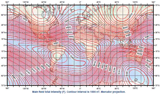

~ 22 years - solar magnetic (Hale) cycle( power peak)

~ 52 & 105 years - sunspot anomalies periods ( power peaks)

~ 20 (19.86)  and & 6-7 (its 3^rd harmonic)  years - Jupiter /Saturn synodic period (power troughs).

~ 60 (59.5,  3^rd sub-harmonic) years - as above but associated with ~ 120 degrees longitudinal shift of the Jupiter /Saturn conjunction shift, when two planets are located in a particularly 'sensitive' part of the heliosphere (e.g. nose or tail end) .

Within the Earth's events, the 20 and particularly 60 year periods are  more pronounced, possibly due to the enhanced magnetic effect when the Earth passes through the particularly strong electro-magnetic link between the sun and the gas giants.

Secular geomagnetic variation as observed at the two  poles in the Northern hemisphere( calculated within + or -5years margin allowing for the NOAA's data gmf resolution):

Siberia  has positive forcing (rising GMF) - peaks:

~ 1940 & ~2000

Hudson Bay negative forcing (falling GMF) - troughs :

 ~1750, ~1810, ~ 1870s, ~1930s, late 1990s.

 

   

Fig. 7 & 8

 

Fig. 9

Total secular variation of the geomagnetic field is combination of the solar induced, ocean currents induction and those due to the Earth's internal dynamics, and can be clearly seen in the correlation with the Central England's temperature records.

http://www.vukcevic.co.uk/HmL.htm

More charts can be found here: Graphs and Formulae

© m.a. vukcevic